|
|
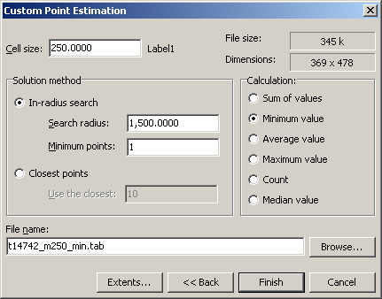
| Figure. A screen shot of the user interface for the Custome Point Estimator. The output grid is set to 250m resolution, the search radius is set to 1500m and the output is the minimum elevation value found within the 1500m search radius for each point. Identical runs are then done for the maximum and median values - the output file names ending in turn with MIN, MAX and MACRO. |
A:
|
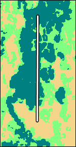
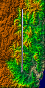
Figure. Examples of the new grids, along a cross-section through Wadbilliga National Park in the south coast of NSW.
|
A:
|
Figure. Examples of calculated grids, along the cross-section through Wadbilliga National Park in the south coast of NSW.
|
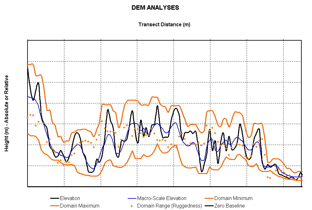 |
Figure. The cross-section, showing the terrain elements discussed above.
|
 B:
B: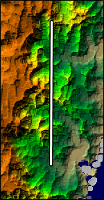 C:
C: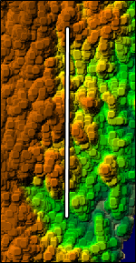 D:
D: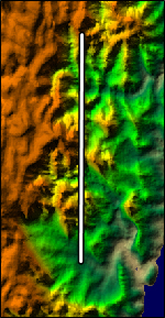
 B:
B: